Predicting academic ability

The paper begins by claiming that the following example shows that selecting parameters for inference based on the data matters for Bayesian inference from one perspective but not from another.

Let \(\theta\) denote students’ true academic ability. The marginal density of \(\theta\) in the population of high school students is \(N(0, 1)\). The observed academic ability of students in high school is \(Y \sim N(\theta, 1)\), and students with \(0 < Y\) are admitted to college. We wish to predict a student’s true academic ability from his observed academic ability — but only if the student is admitted to college. We shall show that the Bayesian inference is different for a random high school student from [the inference] for a random college student.²

For a professor predicting \(\theta\) for a random college student, a Bayesian approach is taken where first the joint distribution of \((\theta, Y)\) for all high school students is found, then the conditional distribution is found for students admitted to college based on \(y > 0\). The result is that given \(Y=y\), the posterior distribution for \(\theta\) is \(N(y/2, 1/2)\), and \(\theta\) could be predicted as \(\hat{\theta}(y) = y/2\). (So far, so good, though the paper doesn’t spell out the important part. If one does the same analysis without conditioning on \(y > 0\) — i.e., if the professor pretends that the student is drawn randomly from the whole high school population — then one arrives at the same result. Thus, the Bayesian analysis is not affected by the filtering on \(y\) which one can view as parameter selection based on the data.)

In contrast, for a high school teacher predicting \(\theta\) for a student in his class, where teachers are allowed to make such a prediction only for students who can be admitted to college (\(y > 0\)), the approach is different. It’s noted that “for any true academic ability \(\theta\), the values of \(Y\) that are used to predict \(\theta\) are drawn from the \(N(\theta, 1)\) density truncated by the event \(0 < Y\).” A joint distribution for \((\theta, y)\) is then derived by combining the truncated normal distribution for \(Y|\theta\) with the \(N(0, 1)\) prior distribution for \(\theta\). The conditional distribution for \(\theta | Y=y\) doesn’t have a closed expression but is known to be shifted downward relative to \(N(y/2, 1/2)\) and thus produces a smaller prediction for \(\theta\) than the professor’s method. (Wait… what?)

---

Why would the college professor and the high school teacher approach the problem differently? For my life, I can’t see what differentiates the two perspectives. In both cases, the same quantity is being predicted for a student from essentially the same population (college-bound or college-admitted students) with the same information about how \(Y\) relates to \(\theta\). Why wouldn’t the high school teacher reason about the problem in exactly the same way as the professor?

Why would the high school teacher use \(N(0, 1)\) for the prior for \(\theta\)? The teacher conditions on \(y > 0\) when determining the distribution of \(Y\) given \(\theta\), but fails to condition the prior distribution of \(\theta\) on \(y > 0\). Thus, the teacher makes the strange assumption that college-bound students have the same true academic abilities as the overall population of high school students despite the filtering according to \(y > 0\). It’s not surprising that the resulting predictions of \(\theta\) are lower than the professor’s predictions for any given \(y\).

The teacher should either (a) limit the analysis to students with \(y > 0\) and recognize that a random student from that population does not represent a draw from \(\theta \sim N(0, 1)\), or (b) perform the analysis as if \(\theta\) were being predicted for every student regardless of \(y\), then simply discard the predictions for students with \(y \leq 0\) — i.e., use the same approach as the college professor.

All this example seems to show is that a Bayesian analysis done based on faulty reasoning will arrive at a different result than an analysis done properly.

If one takes approach (a) above, it can be shown that the resulting posterior distribution of \(\theta\) is the same \(N(y/2, 1/2)\) distribution obtained from the college professor’s perspective. But (b) is obviously simpler.

Looking for clarification

Regarding the potential effect of parameter selection on Bayesian analysis, Yekutieli cites a paper by M. Mandel and Y. Rinott.³ I looked there to see whether it would illuminate Yekutieli’s odd example.

Mandel and Rinott describe a scenario very similar to Yekutieli’s. A scientist comes to a statistician with a request to construct a confidence interval for a binomial probability \(p\). The scientist notes that she and other scientists only ask for a statistician’s help when the binomial experiment has 0 or 1 successes.⁴ Thus, there is a data-based decision of when to carry out inference on the unknown parameter, i.e., parameter selection.

Bayesian analysis is compared between two perspectives. Under Model I, \(p\) is drawn from a prior distribution \(\pi\) once and remains fixed across repeated binomial experiments observing \(X \sim \text{bin}(n, p)\). Under Model II, \(p\) is drawn from \(\pi\) independently for each experiment. The authors prove a couple of mathematical results and derive a Bayesian credible interval for \(p\) under each Model. The two credible intervals turn out to be quite different for an example where \(\pi \sim \text{unif}(0, 1)\) and \(n = 20\).

---

Mandel and Rinott’s findings result from the same error as in the high school teacher’s analysis.

Under Model I, the analysis is performed based on a truncated distribution for \(X|p\), conditioning on \(x \leq 1\). However, the same conditioning on \(x \leq 1\) is not applied to the prior for \(p\), thus resulting in a nonsensical analysis. The scenario is easily simulated to illustrate the error.

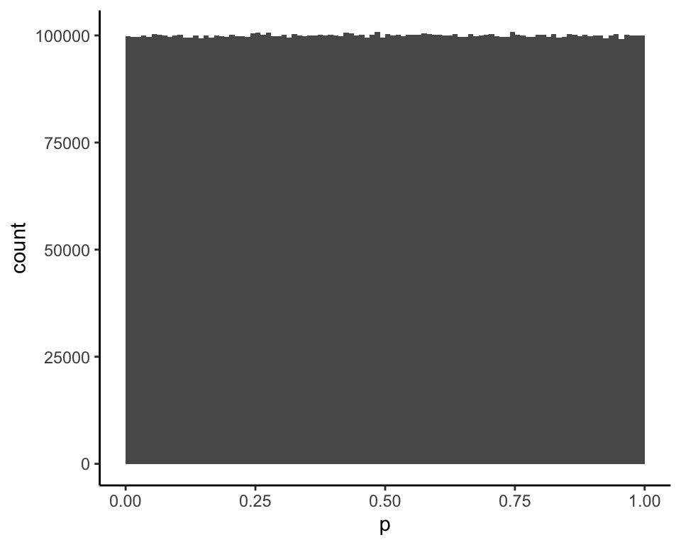
If this is the unif\((0, 1)\) prior distribution for \(p\)…

and the conditional distribution of \(X|p\) for \(n = 20\) is obtained by conditioning on \(x \leq 1\) (rightmost columns)…

p	Pr(X=0)	Pr(X=1)	Pr(X=0 | X in {0,1})	Pr(X=1 | X in {0,1})
(0.01,0.02]	0.74	0.22	0.77	0.23
(0.03,0.04]	0.49	0.35	0.58	0.42
(0.09,0.1]	0.14	0.28	0.32	0.68
(0.19,0.2]	0.01	0.06	0.17	0.83

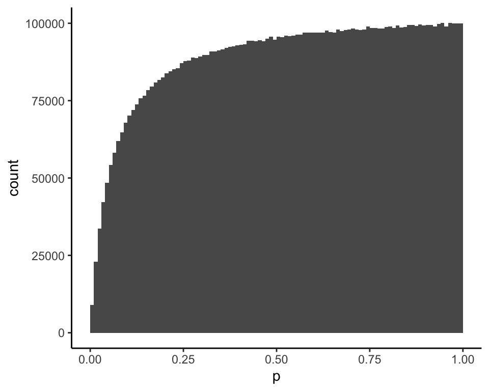
then this is the posterior distribution of \(p\) given \(x = 0\) (mean = 0.18):

and this is the posterior distribution of \(p\) given \(x = 1\) (mean = 0.54):

The 95% credible intervals calculated in the paper are (0.0029, 0.6982) for \(x = 0\) and (0.0620, 0.9778) for \(x = 1\). My simulation finds the same values from the 2.5% and 97.5% percentiles of the posterior distributions:

##        2.5%       97.5% 
## 0.002928565 0.697992157

##       2.5%      97.5% 
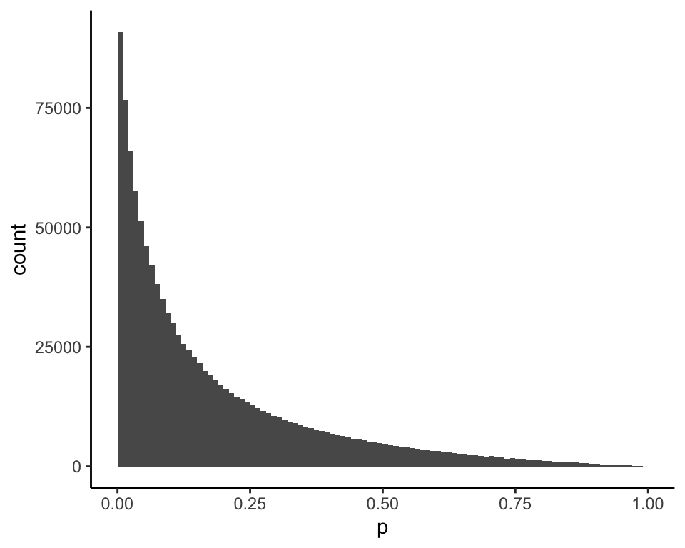
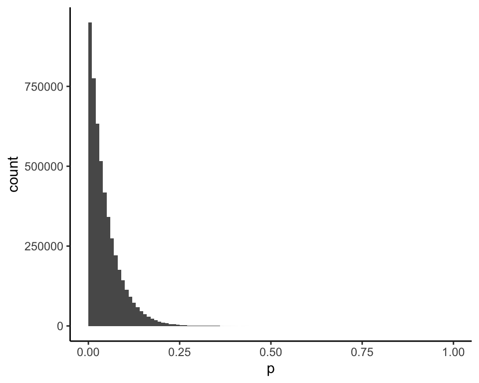
## 0.06198153 0.97780242

However, if you’re going to use the distribution of \(X|p\) conditional on \(x \leq 1\), then a valid Bayesian calculation requires that the prior for \(p\) also be conditional on \(x \leq 1\). The correct prior looks like this (mean = 0.07):

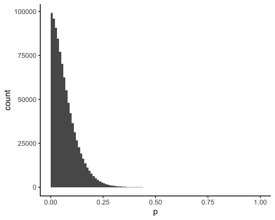
Using the correct prior, this is the posterior distribution of \(p\) given \(x = 0\) (mean = 0.05):

and this is the posterior distribution of \(p\) given \(x = 1\) (mean = 0.09):

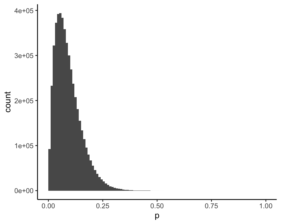
The standard Bayesian analysis for \(p \sim \text{unif}(0, 1)\), \(X|p \sim \text{bin}(n, p)\), and \(n = 20\), which is the same as the authors’ analysis under Model II, gives the same posterior for \(x = 0\) (mean = 0.05):

and for \(x = 1\) (mean = 0.09):

Under Model I, a Bayesian analysis that properly accounts for the filtering on \(x \leq 1\) has the same result as the analysis that ignores the filtering. In this case, as with the prediction of students’ academic ability, Bayesian analysis does not need to be modified to account for the parameter selection.

However, there is information that could alter the Bayesian analysis under Model I. For example, suppose the scientist tells the statistician that she has done 1,000 binomial experiments to investigate this same parameter \(p\), and only one of them resulted in \(x \leq 1\). Incorporating that information would surely adjust the posterior for \(p\) upward.

Conclusions

As far as I can tell, these examples do not show that Bayesian analysis is affected by parameter selection as the authors claim. They only show that one must think carefully about the prior distribution.

A paper by S. Senn⁵ provides some more illuminating examples. There, Bayesian analysis continues not to be affected by parameter selection. However, one example shows that when there is correlation among a set of parameters, observations related to non-selected parameters can contain information about selected parameters (e.g., parameters identified as most “interesting” or “significant” based on the data). My comment at the end of the previous section is related to this. Even in this situation, I wouldn’t say that Bayesian analysis is affected by parameter selection — it just needs to use all of the relevant information.

It may be that there are situations where parameter selection matters, but after looking at these examples, I’m led to believe that in many cases it can be ignored. That would be good news for two-stage statistical analysis where Bayesian analysis is applied to findings that arise from a “screening” process. Bayesian analysis could proceed in a fairly straightforward manner without a need to specify and account for the screening process.