ROC curves and AUROC

First, a quick review of the problem setting. Some type of score, the values of which can be unambiguously ordered from lowest to highest, is measured or calculated from each patient in a population. The purpose of the score is to represent, or correlate with, a patient’s risk of having a particular disease. A reference (“gold”) standard method is used to determine each patient’s disease status.

An ROC curve is constructed by computing the true positive fraction (TPF) and false positive fraction (FPF) for each possible threshold of the score, where the threshold is used to classify patients as “positive” (higher scores) vs “negative” (lower scores).

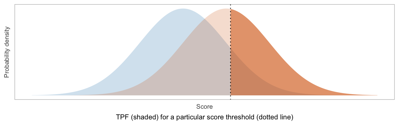
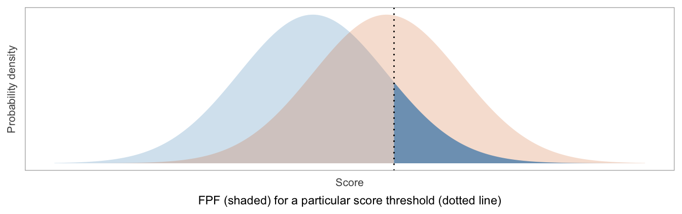
TPF is the same as sensitivity, and FPF is the same as \(1-\)specificity:

TPF = Sensitivity = fraction of patients labeled as positive, among those with disease

FPF = \(1-\)Specificity = fraction of patients labeled as positive, among those without disease

## Warning: A numeric `legend.position` argument in `theme()` was deprecated in ggplot2
## 3.5.0.
## ℹ Please use the `legend.position.inside` argument of `theme()` instead.
## This warning is displayed once every 8 hours.
## Call `lifecycle::last_lifecycle_warnings()` to see where this warning was
## generated.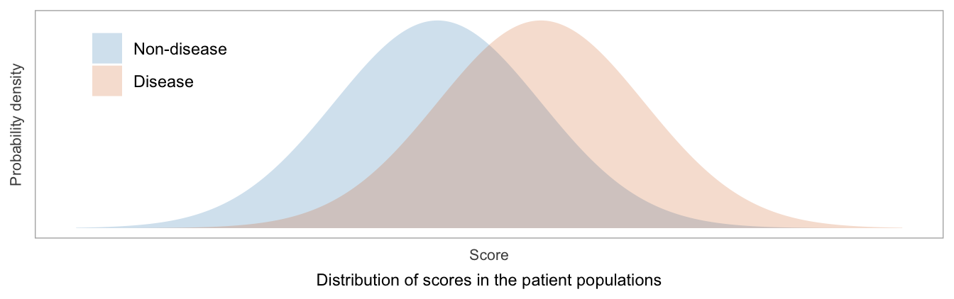

The ROC curve is formed from plotting TPF vs FPF. As the score threshold decreases, the TPF and FPF each increase from 0 to 1. In terms of (FPF, TPF) coordinates, the ROC curve goes from (0, 0) to (1, 1).

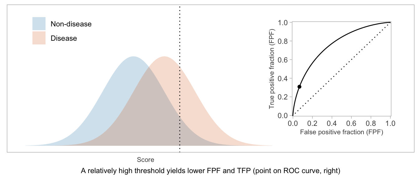
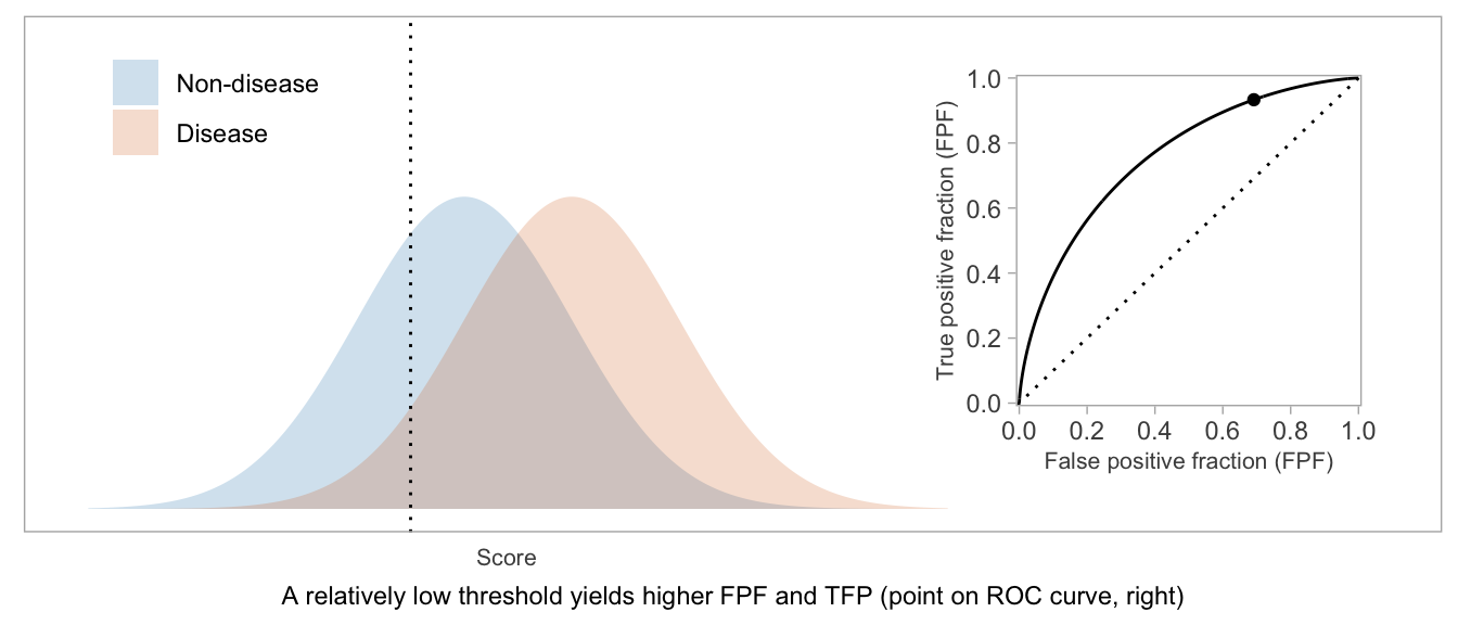
If a score will be used in a dichotomous manner (positive vs negative), the ROC curve can be used as a visual aid in weighing TPF vs FPF and choosing a desirable threshold.

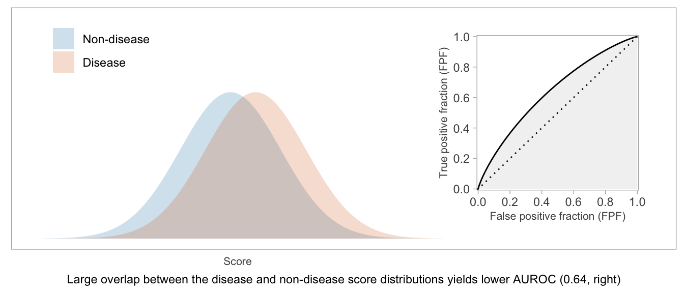
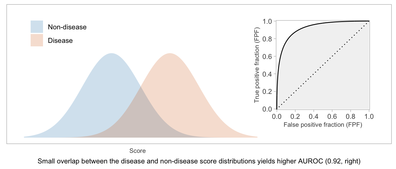
If a score will be used as-is, without dichotomization, or if there’s not yet an accepted threshold for positive classification, then the whole curve is potentially relevant. The AUROC — which is exactly what the name suggests: the area between the \(x\)-axis and the (FPF, TPF) curve — is a way to summarize the curve and condense the (FPF, TPF) values into a single number.

Higher AUROC is desirable. AUROC = 0.5 indicates a useless score, and AUROC = 1 indicates a score that can perfectly separate disease from non-disease patients.

Two interpretations

In the book cited above, Pepe writes,³

The AUC has an interesting interpretation. It is equal to the probability that test results from a randomly selected pair of diseased and non-diseased subjects are correctly ordered, namely \(P[Y_D > Y_{\overline{D}}]\)… Although the interpretation of the AUC as the probability of ‘correctly ordering diseased and non-diseased subjects’ is interesting, it does not necessarily provide the best interpretation of this summary measure. The clinical relevance of the correct ordering is not particularly compelling for the applications that we consider… We prefer to interpret the AUC as an average TPF, averaged uniformly over the whole range of false positive fractions in (0,1).

The interpretation of AUROC as concordance probability is contrasted with an interpretation as an average TPF (sensitivity). While both interpretations are equally correct in a mathematical sense, non-mathematical people may find one view more meaningful than the other, so I’m glad to have come across these passages in the book.

For my own understanding, I found a view of the AUROC in which the equivalence of the two interpretations is so apparent that there’s hardly any need to distinguish between them.

Equivalence of the two interpretations

The scheme above for connecting AUROC to the concordance probability requires only a slight modification to link it to the “average sensitivity” interpretation.

Simply imagine grouping the sampled pairs of patients by their FPF (\(x\)) coordinates after mapping them to the (FPF, TPF) coordinate space. For any given group, suppose the non-disease patients all have scores approximately equal to \(s\); the proportion of concordant pairs in that group is the proportion of disease patient scores greater than \(s\), which is the TPF for threshold \(s\). An average of those proportions, across different values of \(s\), is the same as the overall proportion of concordant pairs because each FPF-based group will have, on average, the same number of patient pairs.

Thus, the calculation of concordance probability is essentially the same as the calculation of average TPF in this scheme, and both are equal to the AUROC.

Formal proof

The equivalence of AUROC, average TPF, and the concordance probability can be formally shown in a straightforward manner that, in some ways, mimics the scheme above:

Consider the ROC curve drawn in \((x, y)\) coordinates, with \(x \in [0, 1]\) and \(y \in [0, 1]\). The ROC curve is a function of \(x\), say \(g(x)\). By definition,

\[\begin{equation} \text{AUROC} = \int_0^1 g(x) dx \end{equation}\]

Let \(F_S(s) = \text{P}(S \leq s)\) be the cdf for non-disease patient scores, \(S\) being a randomly drawn non-disease patient score. Let \(F_T(t) = \text{P}(T \leq t)\) be the cdf for disease patient scores, \(T\) being a random disease patient score. Then again by the definition of ROC curve, as the TPF for a given FPF, \(g(x) = \text{P}(T > s)\) for the score \(s\) which satisfies \(\text{P}(S > s) = x\), i.e. \(1 - F_S(s) = x\). Therefore, \(s = F_S^{-1}(1 - x)\) and

\[\begin{equation} g(x) = 1 - F_T(F_S^{-1}(1 - x)) \end{equation}\]

In the integral for the AUROC,

\[\begin{equation} \text{AUROC} = \int_0^1 \left[ 1 - F_T(F_S^{-1}(1 - x)) \right] dx \end{equation}\]

we change variable from \(x\) to \(s = F_S^{-1}(1 - x)\):

\[\begin{align} \text{AUROC} &= \int_{\infty}^{-\infty} \left[ 1 - F_T(s) \right] [-dF_S(s)] \\ &= \int_{-\infty}^{\infty} \left[ 1 - F_T(s) \right] dF_S(s) \end{align}\]

It follows that

\[\begin{align} \text{AUROC} &= \int_{-\infty}^{\infty} \text{P}(T > s) dF_S(s) \\ &= \int_{-\infty}^{\infty} \text{P}(T > s | S = s) dF_S(s) \\ &= \text{P}(T > S) \end{align}\]

which is the concordance probability. The second line is due to the independence of \(S\) and \(T\) (and also expresses AUROC as an average TPF).

Therefore, AUROC = average TPF = concordance probability.